Research Article - International Research Journal of Engineering Science, Technology and Innovation ( 2025) Volume 11, Issue 2
Received: 29-Aug-2024, Manuscript No. irjesti-24-146849; Editor assigned: 02-Sep-2024, Pre QC No. irjesti-24-146849; Reviewed: 16-Sep-2024, QC No. irjesti-24-146849; Revised: 14-Apr-2025, Manuscript No. irjesti-24-146849; Published: 21-Apr-2025, DOI: 10.14303/2315-5663.2025.125
A resistivity survey was carried out to study groundwater potential in Rumuogolu road of Rukpokwu community, Rivers State of Nigeria with the aim of determining the depth, thickness, resistivity and lithology at which groundwater can be obtained. Four vertical electrical soundings were conducted using the Schlumberger configuration. The VES data were subjected to an iteration software (IPI2WIN) which showed that the area is composed of alluvium sand, sand and sandstone (consolidated). Based on the interpretation, layer under the geoelectric section is sand (made up of fine–coarse sand) in VES05 to VES08 all had four aquiferous zones. The aquifers where good quality groundwater was obtainable were dependent on their depths and thickness of the sand body.
Resistivity survey, Groundwater potential, Four vertical electrical soundings, Iteration software, Geoelectric section
Water is essential to all forms of life, including humans, animals, and plants, but it also depends on the environment's capacity to supply water of a particular quality (Adagunodo TA et al., 2017). It follows that as long as life on Earth persists, water will always be a valuable resource that should not be taken for granted (Fadele SI et al., 2013). Groundwater quality is impacted by both natural and industrial processes (Haider H et al., 2017). Pollution from multiple sources has a considerable impact on water quality. Microorganisms and inorganic chemicals are widely found in human contexts (Nwankwo CN et al., 2013). Therefore, the presence of contaminants beyond WHO criteria can cause a number of ailments, such as typhoid fever, paratyphoid fever, dysentery, gastroenteritis, infectious hepatitis, schistosomiasis, asiatic cholera, back pain, pneumonia, and nasal congestion (Offodile ME, 1992). Water, a natural resource, will continue to be challenged by competition for it in the industrial, agricultural, and hydropower sectors of the global economy (Ojelabi E et al., 2001). This includes dry and semi-arid regions of the world. It is becoming more and more difficult to supply an adequate amount of high-quality water due to population expansion, irrigation, and industrialization (Sajil Kumar PJ et al., 2014).
Surface water cannot be depended upon year-round due to the previously described problems; hence, in different parts of the world, alternative methods are needed to augment surface water. Water is a rare natural resource, despite its importance. Building is not feasible. The hydrologic cycle is the mechanism by which water is renewed through the atmosphere. Subsurface water that fills soil pores and fissures in rock formations is known as groundwater, and it generates around 95% of all water.
As its name implies, groundwater is the water that is found below the earth's surface. Researchers claim that this freshwater is the best available and most sought-after for use worldwide. It is the water that is kept in the saturated zone of the subsurface by hydrostatic pressure beneath the water table. The groundwater may be in basement complex terrain, where it may be more difficult to discover, especially in areas where crystalline rocks are present, or sedimentary terrain, where it may be easier to access. In Rukpowu and the surrounding areas of Southern Nigeria, groundwater is the main source of drinkable water.
Groundwater is usually stored in aquifers. A subterranean water formation that is saturated and has the capacity to supply a well with enough water is called an aquifer. There are two types of aquifers based on their physical characteristics. An aquifer that lacks an impermeable layer directly above the saturation zone is said to be unconfined. An aquifer that is restricted has layers of impermeable materials encircling the saturation zone. An aquifer can usually provide a well or spring with a commercially feasible amount of water. Formation strata and terrain type significantly influence aquifer characteristics. Therefore, adequate and reliable empirical evidence is the only basis for the purchase of commercially viable deep-water wells.
In order to address the problem of water scarcity in Rukpowu, Rivers State, Nigeria, caused by population increase and industrialization, it will be imperative to focus on the identification of groundwater zones and aquifers. The resistivity method of groundwater exploration becomes essential in this context. Groundwater research and water quality evaluations are increasingly using geophysical approaches because of the rapid development of computer software and other numerical modeling tools. Vertical Electrical Sounding (VES) has gained popularity in groundwater prospecting due to its ease of usage. Finding the surface effects of the internal electric current flow of the earth is the aim of the electrical geophysical survey approach. These techniques have been used in many different geophysical investigations, including as mineral exploration, archeological study, engineering studies, geothermal exploration, permafrost mapping, and geological mapping.
Proper groundwater exploration requires deep and comprehensive methodologies to collect critical data on the distribution, thickness, and depth of groundwater-bearing formation. Some of the surface geophysical techniques used in groundwater investigations are the electrical resistivity method, seismic refractive method, magnetic method, radioactivity method, gravity method, and electromagnetic method. According to Adagunodo et al., these techniques can map the topography and architecture of bedrock in addition to the thickness of the aquiferous zones and overburden.
Resistivity techniques are utilized not only to identify 3D objects with aberrant conductivity, but also to analyze vertical and horizontal variations in the electrical characteristics of the ground. The resistivity approach uses the resistive method to record the potential differences at the surface by injecting artificially generated electrical currents into the ground. It is frequently employed to investigate the shallow subsurface geology in hydrogeology and engineering studies. Variations in the pattern of the potential differences predicted from homogeneous ground can be used to assess the structure and electrical properties of sub-surface in homogenicity.
The hydrological conditions of the region, the resistivity and thickness of the subsurface layers, and the optimal sites for borehole drilling within the study area were all examined in this study.
Geology and hydrogeology of the study area
The sediments that comprise Rukpokwu are derived from the strata of the Niger Delta complex. This group of sedimentary basins in southern Nigeria is referred to as the "Cenozoic Formation". The Niger Delta sedimentary basin's sedimentary deposits range in thickness from 9,000 to 12,000 meters. Most of these sediments are lenticular and unconsolidated, while a small percentage are slightly sorted and poorly cemented. Above the sedimentary succession is a thick layer of ferruginized and weathered red earth from previous sequences. Due to the area's excellent hydrological conditions, including the substantial annual rainfall, aquifers can form (Figure 1).

Figure 1. Location map showing sounding points at Rukpokwu.
The study team used the ABEM SAS 1000 terra meter and its attachments to explore below ground, utilizing Schlumberger electrodes in four profiles (average distance of 100 meters), they separated the electrodes at 0.60 meters, 30 meters, 400 meters, and 200 meters utilizing the vertical electrical sounding approach. Equation 1, the SAS 1000, and its accessories allowed them to measure apparent resistivity at four different locations across the study area.
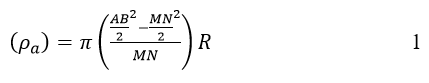
The equation is simplified as in Equation (2)
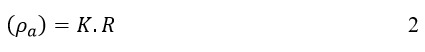
where the geometric factor
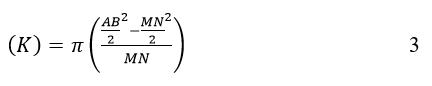
MN is the potential electrode separation, R is the measured resistance, and AB is the current. By measuring the impact of the current injected beneath the surface of the ground, the earth resistance was ascertained. Geometrically, the measured resistance is multiplied by the geometric component k of the electrode design (Figure 2 and Tables 1-4).

Figure 2. The Schlumberger electrode configuration used in the study area.
| S/N | AB/2(m) | MN/2(m) | Geometric facctor (K) | Resistance (r) | Apparent resistivity (ρa) |
| 1 | 1.00 | 0.30 | 4.76 | 132.52 | 630.79 |
| 2 | 2.00 | 0.30 | 20.47 | 36.305 | 743.16 |
| 3 | 3.00 | 0.30 | 46.65 | 16.316 | 761.14 |
| 4 | 4.00 | 0.30 | 83.30 | 8.5614 | 713.25 |
| 5 | 4.00 | 0.50 | 49.48 | 15.253 | 754.71 |
| 6 | 6.00 | 0.50 | 112.31 | 5.3332 | 599.02 |
| 7 | 7.00 | 0.50 | 153.15 | 5.3950 | 826.35 |
| 8 | 8.00 | 0.50 | 200.27 | 5.0852 | 1018.56 |
| 9 | 8.00 | 1.00 | 98.96 | 10.206 | 1010.08 |
| 10 | 10.00 | 1.00 | 155.50 | 1.2422 | 1126.30 |
| 11 | 15.00 | 1.00 | 351.85 | 12.315 | 4333.64 |
| 12 | 15.00 | 1.55 | 233.26 | 14.486 | 3379.43 |
| 13 | 20.00 | 1.50 | 416.52 | 15.272 | 6361.85 |
| 14 | 25.00 | 1.50 | 652.14 | 4.8123 | 3138.67 |
| 15 | 25.00 | 2.50 | 388.77 | 6.7286 | 2616.21 |
| 16 | 30.00 | 2.50 | 561.55 | 13.114 | 7365.21 |
| 17 | 40.00 | 2.50 | 1001.38 | 13.898 | 13918.98 |
| 18 | 50.00 | 2.50 | 1566.86 | 6.2869 | 9852.01 |
| 19 | 50.00 | 5.00 | 777.54 | 7.2524 | 5639.79 |
| 20 | 80.00 | 7.50 | 1328.63 | 1.2632 | 2530.21 |
| 21 | 100.00 | 10.00 | 1555.08 | 181.55 | 282.28 |
| 22 | 150.00 | 15.00 | 2332.63 | 1.5611 | 3641.93 |
| 23 | 200.00 | 15.00 | 4165.22 | 1.0948 | 4560.67 |
Table 1. Numerical representation of apparent resistivity for VES05.
| S/N | AB/2 (m) | MN/2 (m) | Geometric facctor (K) | Resistance (r) | Apparent resistivity (Pa) |
| 1 | 1.00 | 0.30 | 4.76 | 190.23 | 888.37 |
| 2 | 2.00 | 0.30 | 20.47 | 57.587 | 1178.80 |
| 3 | 3.00 | 0.30 | 46.65 | 29.178 | 1361.15 |
| 4 | 4.00 | 0.30 | 83.30 | 15.872 | 1322.29 |
| 5 | 4.00 | 0.50 | 49.48 | 27.485 | 1359.95 |
| 6 | 6.00 | 0.50 | 112.31 | 13.172 | 1479.47 |
| 7 | 7.00 | 0.50 | 153.15 | 10.249 | 1569.83 |
| 8 | 8.00 | 0.50 | 200.27 | 6.7355 | 1349.46 |
| 9 | 8.00 | 1.00 | 98.96 | 14.110 | 1396.46 |
| 10 | 10.00 | 1.00 | 155.50 | 10.594 | 1647.57 |
| 11 | 15.00 | 1.00 | 351.85 | 5.3077 | 1865.66 |
| 12 | 15.00 | 1.50 | 233.26 | 7.452 | 1738.47 |
| 13 | 20.00 | 1.50 | 416.52 | 5.2801 | 2199.53 |
| 14 | 25.00 | 1.50 | 652.14 | 6.1414 | 4005.54 |
| 15 | 25.00 | 2.50 | 388.77 | 8.3258 | 3237.23 |
| 16 | 30.00 | 2.50 | 561.55 | 8.2181 | 4615.53 |
| 17 | 40.00 | 2.50 | 1001.38 | 2.7692 | 2773.38 |
| 18 | 50.00 | 2.50 | 1566.86 | 1.7605 | 2758.82 |
| 19 | 50.00 | 5.00 | 777.54 | 3.1564 | 2454.55 |
| 20 | 70.00 | 5.00 | 1531.52 | 3.8262 | 5860.66 |
| 21 | 80.00 | 5.00 | 2002.76 | 7.2277 | 14477.22 |
| 22 | 80.00 | 7.50 | 1328.63 | 7.1387 | 9485.90 |
| 23 | 100.00 | 7.50 | 2082.61 | 4.2206 | 8791.00 |
| 24 | 100.00 | 10.00 | 1555.08 | 5.3966 | 8393.27 |
| 25 | 150.00 | 10.00 | 3518.58 | 2.7404 | 9638.09 |
| 26 | 150.00 | 15.00 | 2332.63 | 3.1502 | 7349.19 |
| 27 | 200.00 | 15.00 | 4165.22 | 6.1848 | 25764.39 |
Table 2. Numerical representation of apparent resistivity for VES06.
| S/N | AB/2 (m) | MN/2(m) | Geometric facctor (K) | Resistance (R) | Apparent resistivity (Pa) |
| 1 | 1.00 | 0.30 | 4.76 | 130.65 | 621.89 |
| 2 | 2.00 | 0.30 | 20.47 | 42.247 | 864.79 |
| 3 | 3.00 | 0.30 | 46.65 | 22.761 | 1061.80 |
| 4 | 4.00 | 0.30 | 83.30 | 13.110 | 1092.19 |
| 5 | 4.00 | 0.50 | 49.48 | 21.038 | 1040.96 |
| 6 | 6.00 | 0.50 | 112.31 | 10.778 | 1210.58 |
| 7 | 7.00 | 0.50 | 153.15 | 7.2924 | 1116.97 |
| 8 | 8.00 | 0.50 | 200.27 | 5.2369 | 1048.95 |
| 9 | 8.00 | 1.00 | 98.96 | 10.077 | 997.32 |
| 10 | 10.00 | 1.00 | 155.50 | 7.6223 | 1185.42 |
| 11 | 15.00 | 1.00 | 351.85 | 7.0358 | 2475.89 |
| 12 | 15.00 | 1.50 | 233.26 | 9.6499 | 2251.22 |
| 13 | 20.00 | 1.50 | 416.52 | 3.2586 | 1357.43 |
| 14 | 25.00 | 1.50 | 652.14 | 4.3243 | 2820.39 |
| 15 | 25.00 | 2.50 | 388.77 | 5.4959 | 2136.91 |
| 16 | 30.00 | 2.50 | 561.55 | 6.1730 | 3466.94 |
| 17 | 40.00 | 2.50 | 1001.38 | 8.22551 | 8237.51 |
| 18 | 50.00 | 2.50 | 1566.86 | 2.7897 | 4371.65 |
| 19 | 50.00 | 5.00 | 777.54 | 4.0871 | 3178.31 |
| 20 | 70.00 | 5.00 | 1531.52 | 11.509 | 11628.56 |
| 21 | 80.00 | 5.00 | 2002.76 | 3.3529 | 6715.92 |
| 22 | 80.00 | 7.50 | 1328.63 | 1.7644 | 2344.53 |
| 23 | 100.00 | 7.50 | 2082.61 | 1.0307 | 2146.82 |
| 24 | 100.00 | 10.00 | 1555.08 | 1.3372 | 2079.73 |
| 25 | 150.00 | 10.00 | 1000.00 | 1.43929 | 1439.29 |
| 26 | 200.00 | 15.00 | 4165.22 | 4.6611 | 19417.02 |
Table 3. Numerical representation of apparent resistivity for VES07.
| S/N | AB/2 (m) | MN/2(m) | Geometric facctor (K) | Resistance (R) | Apparent resistivity (Pa) |
| 1 | 1.00 | 0.30 | 4.76 | 241.66 | 1150.30 |
| 2 | 2.00 | 0.30 | 20.47 | 65.022 | 1331.00 |
| 3 | 3.00 | 0.30 | 46.65 | 21.381 | 997.42 |
| 4 | 4.00 | 0.30 | 83.30 | 17.165 | 1430.01 |
| 5 | 4.00 | 0.50 | 49.48 | 28.899 | 1429.92 |
| 6 | 6.00 | 0.50 | 112.31 | 10.742 | 1206.54 |
| 7 | 7.00 | 0.50 | 153.15 | 6.2739 | 960.97 |
| 8 | 8.00 | 0.50 | 200.27 | 6.2683 | 1255.54 |
| 9 | 8.00 | 1.00 | 98.96 | 12.848 | 1271.56 |
| 10 | 10.00 | 1.00 | 155.50 | 7.7170 | 1200.14 |
| 11 | 15.00 | 1.00 | 351.85 | 9.0707 | 3171.00 |
| 12 | 15.00 | 1.50 | 233.26 | 11.376 | 2653.90 |
| 13 | 20.00 | 1.50 | 416.52 | 7.9463 | 3101.90 |
| 14 | 25.00 | 1.50 | 652.14 | 4.5718 | 2981.81 |
| 15 | 25.00 | 2.50 | 388.77 | 6.6209 | 2574.33 |
| 16 | 30.00 | 2.50 | 561.55 | 3.0405 | 1707.63 |
| 17 | 40.00 | 2.50 | 1001.38 | 3.4171 | 3422.25 |
| 18 | 50.00 | 2.50 | 1566.86 | 3.8796 | 6079.60 |
| 19 | 50.00 | 5.00 | 777.54 | 5.1337 | 3992.19 |
| 20 | 70.00 | 5.00 | 1531.52 | 2.1981 | 366.87 |
| 21 | 80.00 | 5.00 | 659.20 | 1.25 | 824.64 |
| 22 | 80.00 | 7.50 | 1328.63 | 1.8232 | 2422.66 |
| 23 | 150.00 | 10.00 | 3518.58 | 28.584 | 100588.2 |
Table 4. Numerical representation of apparent resistivity for VES08.
Field data processing
The field data from the VES was processed using the resistivity sounding analysis application (IPI2WIN) to determine the true resistivity and depth of the subsurface formations. This software is 3.0 version. The computer program creates model curves automatically using the starting layer parameters of resistivity and thickness that are derived from the partial curve match of the field curve with standard curves. The true layer parameters for the geo-electric section are calculated, and the outcomes are displayed for the place in terms of resistivities and geoelectric depth.
The resulting model curves have RMS errors less than 5% IN VES 5 and VES 8 and more than 5% in VES 6 and VES 7 curves with four (4) interpretable geoelectric layers for all VES stations, the obtained curves are Hk and Ak for all VES stations. The results are of the form of figures and tables (Figures 3-10 and Tables 5-8).

Figure 3. VES 5.
| Layers | Resistivity | Depth (m) | Thickness (m) | Lithology |
| 1 | 690.0 | 2.3 | 2.3 | Alluvium sand |
| 2 | 1056.6 | 15.1 | 17.4 | Sand |
| 3 | 6288.9 | 17.2 | 34.6 | Sandstone (consolidated) |
| 4 | 1119.3 | - | - | Sandstone (consolidated) |
Table 5. Resistivity and depth of VES 5.

Figure 4. Lithologic log and interpreted geoelectric sections with depth.

Figure 5. VES 6.
| Layers | Resistivity | Depth (m) | Thickness (m) | Lithology |
| 1 | 606.0 | 0.4 | 0.4 | Alluvium sand |
| 2 | 1435.0 | 6.7 | 7.1 | Sand |
| 3 | 3196.0 | 8.0 | 15.1 | Sandstone (consolidated) |
| 4 | 2630.0 | - | - | Sandstone (consolidated) |
Table 6. Resistivity and depth of VES 6.

Figure 6. Lithologic log and interpreted geo-electric sections with depth.

Figure 7. VES 7.
| Layers | Resistivity | Depth (m) | Thickness (m) | Lithology |
| 1 | 804.0 | 2.0 | 2.0 | Alluvium sand |
| 2 | 1576.2 | 23.3 | 25.3 | Sand |
| 3 | 4642.6 | 17.0 | 42.3 | Sandstone (consolidated) |
| 4 | 1174.0 | - | - | Sandstone (consolidated) |
Table 7. Resistivity and depth of VES 7.

Figure 8. Lithologic log and interpreted geoelectric sections with depth.

Figure 9. VES 8.
| Layers | Resistivity | Depth (m) | Thickness (m) | Lithology |
| 1 | 1360.0 | 1.3 | 1.3 | Alluvium sand |
| 2 | 1185.0 | 9.2 | 10.5 | Sand |
| 3 | 7712.5 | 11.9 | 22.4 | Sandstone (consolidated) |
| 4 | 2700.3 | - | - | Sandstone (consolidated) |
Table 8. Resistivity and depth of VES 8.

Figure 10. Lithologic log and interpreted geoelectric sections with depth.
Interpretation of result
Geologic maps of the Niger Delta place the research site within the Benin formation. This indicates that fine to medium to coarse sand with clay intercalation make up the majority of the lithological units that are expected to be found there. Based on the work of Keller and Frischknecht, the resistivity range is employed for a few specific sedimentary rock components in order to understand the VES data.
Discussion of results
The vertical electrical sounding modeling carried out at four (4) VES stations was used to derive the geo-electric sections of various profile; which indicate the existence of mostly four geologic layers in the study area in each VES point were the survey was carried out. This comprised the top soil, weathered basement, fractured basement and fresh basement rocks. From the study, the top spoil consists of alluvium sand.
Results showed that the first point (VES 5) has AK type curve with four (4) geoelectric layers (ρ1<ρ2<ρ3>ρ4) and the second point (VES 6) has AK type curve with four (4) geoelectric layers (ρ1<ρ2<ρ3>ρ4). The third point (VES 7) has an HK type curve with four (4) geoelectric layers ρ1>ρ2<ρ3>ρ4 and the fourth point (VES 8) has AK curve type (ρ1<ρ2<ρ3>ρ4) of vertical electrical sounding curves respectively. The layers are interbeded with shale, clay, mud and sand since the area of study is situated in the Benin formation.
As presented in Table 5 to Table 8, the following deductions was made. The resistivity values of the study area ranged from 606 Ωm to 1360 Ωm, with an average value of 865 Ωm in the first layer and the second layer has its resistivity values ranging from 1056.6 Ωm to 1576.2 Ωm, with an average value of 1313.2 Ωm. The third layer has its resistivity values ranging from 3196 Ωm to 7712.5 Ωm, with an average value of 5459.99 Ωm, while the fourth layer has its resistivity values ranging from 1119.31 Ωm to 2700.3 Ωm, with an average value of 1905.90 Ωm. The corresponding interpreted layer thickness values range from 0.4 m to 2.3 m for the first layer, 7 m to 25 m for second layer, 15 m to 42 m for third layer and layer four has an infinite thickness, which indicates the availability of portable good water for drinking. Therefore, good potable water can be gotten from a depth of 7 m to 42 m in Rukpokwu community and its environs.
The correlation analysis revealed that the thickness and depth of the aquifer to the basement tended to be higher in areas with high resistivity of the top soil, and lower in areas with low resistivity. Similarly, in terrain with complicated basements, groundwater potential was found to be highest in areas with high levels of overburden. Consequently, groundwater development was most effective in areas with aquifer thickness of 15 m or more. Based on this premise, the groundwater potential was determined to be high in the following areas: VES 05; VES 06; VES 07; VES 08.